Error Analysis in Experimental Physical Science

§5 - Using the Gaussian

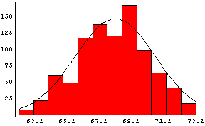
In the previous section we saw examples of data that are distributed at least approximately like a Gaussian. Here we again show the data taken by Galton on heights, this time with a Gaussian curve superimposed on it:

The amplitude of the curve is 146.4, the mean is 68.2, and the standard deviation is 2.49.

Of course, the data do not perfectly match the curve because "only" 928 people were measured.

If we could increase the sample size to infinity, we might expect the data would perfectly match the curve. However there are problems with this:

• For data like the height data, we can not even in principle increase the sample size to infinity since there are not an infinite number of people in the world.
• For data like the radioactive decays which we also looked at in the previous section, it would take an infinite amount of time to repeat the measurements an infinite number of times.
• For many types of data, such as the height data, clearly the assumption of a normal distribution is only an approximation. For example, the Gaussian only approaches zero asymptotically at ± infinity. Thus if the height data is truly Gaussian we could expect to find some people with negative heights, which is clearly impossible! Nonetheless, we will often find that treating data as if it were normally distributed is a useful approximation.

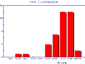
In the previous section we also looked at a distribution of laboratory marks. It is shown again to the right. We imagine that we will ignore the small excess of students with very low marks, since almost all of them have actually dropped the laboratory. We typically would like to know the mean of the other marks so we may know how good the average student is. We would also like to know the standard deviation so we may know how diverse the students are in their laboratory ability.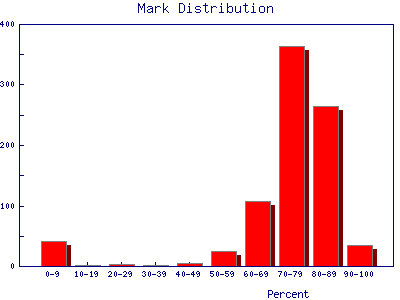

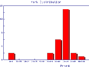
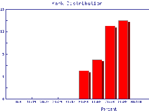
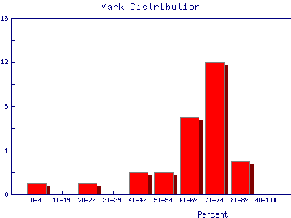
We also may wish to find out the same information for the marks of individual Teaching Assistants to judge student ability and also perhaps to see if the TAs are all marking consistently. Here are the mark distributions for four of the Teaching Assistants in the laboratory.

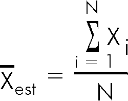
For each of these five mark distributions, it is fairly clear that the limited sample sizes mean that we can only estimate the mean; we will give the estimated mean the symbol . It is calculated by adding up all the individual marks X_i and dividing by the number of marks N.

Similarly, we can only estimate the standard deviation, which we will give the symbol . The statisticians tell us that the best estimate of the standard deviation is:

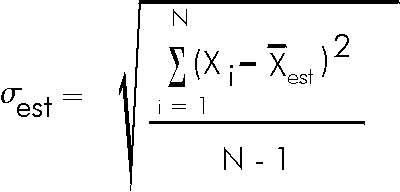
Note that the above equation indicates that can not be calculated if N is one. This is perfectly reasonable: if you have only taken one measurement there is no way to estimate the spread of values you would get if you repeated the measurement a few times.

The quantity N - 1 is called the number of degrees of freedom.

The point we have been making about estimated versus true values of the mean and standard deviation needs to be emphasised:

For data which are normally distributed, the true value of the mean and the true value of the standard deviation may only be found if there are an infinite number of data points.

In the previous section we looked at some data on the number of decays in one second from a radioactive source. Here we shall use this sort of data to explore the estimated standard deviation.

In Question 4.2, you hopefully answered that there is a 68% chance that any measurement of a sample taken at random will be within one standard deviation of the mean. Usually the mean is what we wish to know and each individual measurement almost certainly differs from the true value of the mean by some error. But there is a 68% chance that any single measurement lies with one standard deviation of this true value of the mean. Thus it is reasonable to say that:

The standard deviation is the error in each individual measurement of the sample.

The error in a quantity is usually indicated by a , so the above statement may be written as:

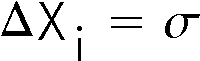
This error is often called statistical. We shall see other types of errors later.

Often what we really want to know is the error in the estimated mean. However, we will need to learn some more about error analysis before we can discuss this topic.

Question 5.1. Listed here are twenty measurements of the time for a stone to fall from a window to the ground, in hundredths of a second.

Compute the estimated mean and the estimated standard deviation of the twenty measurements.

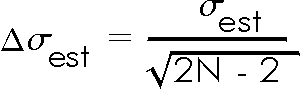
In Exercise 5.1 you saw that the estimated standard deviation was different for each trial with a fixed number of repeated measurements. In fact, if you make a histogram of a large number of trials it will show that these estimated standard deviations are normally distributed. It can be shown that the standard deviation of this distribution of estimated standard deviations, which is the error in each value of the estimated standard deviation, is: Since the estimated standard deviation is the error in each individual measurement, the above formula is the error in the error!

This document is Copyright © 2001, 2004 David M. Harrison

This work is licensed under a Creative Commons License.

This is $Revision: 1.4 $, $Date: 2004/07/18 16:50:40 $ (year/month/day) UTC.