In the physical sciences a specification of an error associated with some quantity essentially defines what the significant figures of that quantity are. By default, LinearFit uses this definition of significant figures in returning the values of the fit parameters. For example, here are the results of a fit of some thermocouple calibration data to a second order polynomial:
| var.names/data.val **** Fit Number 1 **** voltage with error errVoltage versus temp with no error A0 = -0.886 ± 0.030 A1 = 0.0352 ± 0.0014 A2 = 0.000060 ± 0.000013 Chi Squared = 1.0066 for 18 Degrees of Freedom (Chi-squared probability: 100.) |
![[Graphics:../Images/index_gr_112.gif]](../Images/index_gr_112.gif) |
As we shall see soon, in the above fit the intercept A0 is numerically equal to -0.886245 ± 0.0298453 as calculated by the "engine room" of the fitter. This mean that the intercept could be as small as -0.886245 - 0.0298453 = -0.9160903 and it might be as large as -0.886245 + 0.0298453 = -0.8563997. So if the data are good and the we are using a correct model, that the data fits to a second order polynomial, then we are saying that the "true" value of the intercept is probably between -0.9160903 and -0.8563997. Viewed in this way, it seems clear that there is no real significance in the value of the intercept in the ten-thousandth column or any column to its right. Thus, we should say that the "true" value probably lies in the range -0.916 and -0.856. This is equivalent to stating that the intercept is -0.886 ± 0.030, which is exactly the result given above by the fitter.
This is the significant figure adjustment that is the default for LinearFit.
The adjustment can be turned off with the UseSignificantFigures option. The relevant part of the Fit Options screen after turning off significant figure adjustment will look like this:
The result of the fit is now:
| var.names/data.val **** Fit Number 2 **** voltage with error errVoltage versus temp with no error (UseSignificantFigures: False) A0 = -0.886245 ± 0.0298453 A1 = 0.0352394 ± 0.00138311 A2 = 0.0000597878 ± 0.0000133533 Chi Squared = 1.0066 for 18 Degrees of Freedom (Chi-squared probability: 100.) |
![[Graphics:../Images/index_gr_112.gif]](../Images/index_gr_112.gif) |
Now the estimated errors in the fitted parameters have not been used to adjust the number of significant figures displayed for either the values or the errors in those parameters. In the usual case, this is silly.
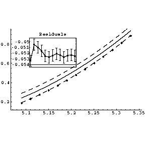
However, there are times when significant figure adjustment does the wrong thing. For example, here is a fit of some data on a free falling object taken by Professor A.W. Key, Dept. of Physics, Univ. of Toronto in December 1999. The fit is to a second order polynomial.
| s with error errs versus
t with error errt A0 = 93.6 ± 1.6 A1 = -38.61. ± 0.60 A2 = 3.982 ± 0.058. Chi Squared = 5.8397 for 10 degrees of freedom. (Chi-squared probability: 82.9267) |
 |
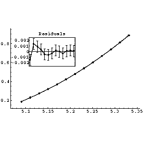
Note that all the residuals are less than zero. Also note that the solid line in the main plot representing the "best" fit is above the data points, and the dashed line representing the minimum fit consistent with the errors in the parameters is the one that goes through the data points. Turning off significant figure adjustment helps considerably:
| s with error errs versus
t with error errt (UseSignificantFigures: False) A0 = 93.5566 ± 1.56078 A1 = -38.6103 ± 0.599245 A2 = 3.98174 ± 0.0575088 Chi Squared = 5.8397 for 10 degrees of freedom. (Chi-squared probability: 82.9267) |
 |
|
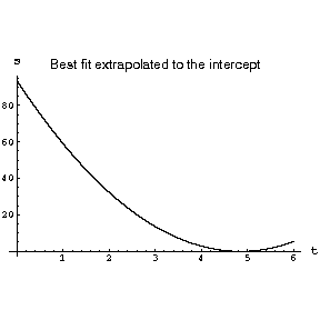
What has happened is that in the original fit, rounding the intercept A0 made all fitted values of the dependent variable systematically almost 0.05 units too high. Note that the value of the intercept itself is huge compared to the experimental values of the dependent variable. This is because, as shown to the right, a plot of the fit results that extrapolates to the intercept shows that the curve "turns over" as the time goes to zero. This, in turn, is a consequence of the fact that the Pasco apparatus used by Professor Key began taking distance measurements at time t = 5.0901 instead of a physically more realistic value of zero. |
 |
Turning off significant figure adjustment can be required in other contexts. For example, a set of synthetic data devised by R.H. Wampler to test linear least-squares fitters such as LinearFit consists of x, y pairs. The certified regression statistics for this data when it is fit to a fifth order polynomial are known and given to a large number of significant figures. In order to compare the results from LinearFit to these values we must turn off significant figure adjustment. The table shows the results of fitting the data to a fifth order polynomial with and without significant figure adjustment, and shows the exact results from Wampler.
| UseSignificantFigures: True | UseSignificantFigures: False | Certified Results |
|---|---|---|
| A0 = 0. ± 2.2 ×
107 A1 = 0. ± 2.4 × 10⁷ A2 = 0. ± 7.8 × 10⁶ A3 = 0. ± 1 × 10⁶ A4 = 0. ± 56000. A5 = 0. ± 1100. |
A0 = 0.997691 ± 2.15233 ×
107 A1 =1.00337 ± 2.36355 × 10⁷ A2 = 0.998935 ± 7.79344 × 10⁶ A3 = 1.00013 ± 1.01476 × 10⁶ A4 = 0.999993 ± 56456.7 A5 = 1. ± 1123.25 |
A0 = 1.00000000000000 ±
21523262.4678170 A1 = 1.00000000000000 ± 23635517.3469681 A2 = 1.00000000000000 ± 7793435.24331583 A3 = 1.00000000000000 ± 1014755.07550350 A4 = 1.00000000000000 ± 56456.6512170752 A5 = 1.00000000000000 ± 1123.24854679312 |
By turning off significant figure adjustment, the result by LinearFit shows good agreement with the certified results.
The United States government National Institutes of Standards and Technology (NIST) has a large collection of data, including the Wampler data, for testing fitters at their web site http://www.nist.gov/itl/div898/strd.
This help document is Copyright © 1999 David M. Harrison. The sample screens are Copyright © 1999 Solomon R.C. Douglas and David M. Harrison. This is version 1.3 of the help document, date (m/d/y) 12/08/99.