Fyzx and Phlash: Using Flash to Demonstrate Physics

Flash is well-known for producing spiffy animations. Not as well-known is how to use it for demonstrations in the sciences using proper mathematical equations to control the motions. Using proper Physics equations for animations is also useful for realistic games. This small document is a tutorial in exploiting the capability of using equations to control animations. I assume that you already know at least a little about using Flash, and have at least a rudimentary knowledge of ActionScript.

We will create 5 different animations below. I have made each of them as simple as possible, so we don't get mired in unimportant details.

When this document was written, the current Flash program was MX 2004. Some discussion of defaults below assumes this version.

The Undamped Harmonic Oscillator

We will use a harmonic oscillator, such as a mass oscillating on a spring, as our example. The mathematics is fairly simple. For the ideal case of an oscillator with no dissipative forces, the motion is given by:

(1)

A is the maximum amplitude of the oscillation.

(pronounced omega naught) is the "natural" angular frequency of oscillation, and depends on the mass and the particular spring. t is the time.

(pronounced phi) is called the "phase angle" of the oscillation, and essentially depends on what moment in time we choose to call zero.

In this document we will be clever and choose the phase angle to be zero. Thus, we will do an animation that obeys the following equation:

(2)

Although we call the position y, below we will find it convenient to have the motion occur in the horizontal direction. In ActionScript-speak, this is named _x.

Above the angular frequency is measured in radians/second, which when multiplied by the time gives radians. Flash trig functions also measure angles in radians. Usually humans think about such motion in terms of the frequency, measured in Hz, or the period T of oscillation. The period is related to the angular frequency by:

(3)

To the right we show a plot of Eqn. 2 for a value of the period equal to 2 seconds.

Faking It

Although this tutorial is primarily about using ActionScript to properly control an animation, sometimes it is possible to do pretty well by faking it. That is the topic of this section.

Our undamped oscillator will have a period of 2.0 seconds. This corresponds to an angular frequency equal to (pronounced pi), which is irrational.

I like to write to the minimum level of the Flash player possible. This minimises the number of people who have to update their player to view the animation. For this project, that means I would change the Settings ... to Flash Player 5. Perhaps for you this is not important, and you can leave the settings to the default (Flash Player 7, ActionScript 2) if you prefer.

Open a new Flash document and place some object, such as a circle, on the stage. Insert key frames at frames 7, 13, 19 and 25. A portion of your Flash window should now look similar to this:

Above we said that we wanted a period of 2.0 seconds, and at the default Flash frame rate of 12.0 fps this corresponds to 24 frames. You may be wondering why we set the last key frame at frame 25 instead of 24. The reason is that the first frame is 1, not 0. Thus between the first and last key frame is 25 -1 = 24 frames. Similarly, from any key frame to the next is exactly 6 frames, which is 1/4 of the period.

We will have the object in key frames 1, 13 and 25 be the equilibrium position, and will not change the position of the object in these frames.

Choose the key frame at frame 7 and move the object some distance to the right. Choose the key frame at frame 19 and move the object the same distance to the left.

Now, put a tween between each pair of key frames. My object is just a circle, so I used a Shape tween. The result looks like this:

This is not good. It doesn't look very harmonic, and there is a "bump" when it moves through the center position from the left to the right.

To make it look more realistic, we will use Eases on the tweens. The Ease control is just under the Tween one in the Properties panel. After selecting a tween, the figure to the right shows setting an "Ease Out 100."

Set the following Eases:

Between Frames 1 & 7: Ease Out 100.
Between Frames 7 and 13: Ease In 100.
Between Frames 13 and 19: Ease Out 100.
Between Frames 19 and 25: Ease In 100.

Finally, the "bump" is because both key frames 1 and 25 have the object in the same position. To fix:

Insert a key frame at frame 24. Be sure to do this only after all the tweens have been made and eased.
In frame 25, remove the contents and remove the frame. Now the final frame of the animation is 24.

The result looks like this:

This looks pretty good, and may in fact be good enough for your purposes.

You may want to take a moment and convince yourself that the period of this last animation is 2.00 seconds. In fact the first animation above had an a period equal to 25/12 = 2.083 seconds. In general I would have preferred for Flash to begin counting the frames from 0, not 1.

Doing It With ActionScript

Now we will do a similar animation to above using the ActionScript language that is built in to Flash. As before the oscillator will have a period of 2.00 sec. You will see that this animation has only one frame.

The ActionScript language has similar syntax to C, JavaScript, etc. so if you know one of those languages you already know where to put the curly braces, semi-colons etc. You will also see that we use the math functions and constants of Flash; these begin with the string Math., such as Math.sin().

Create a new Flash document. I changed the Settings to Flash Player 6, and ActionScript 1, but you can use the defaults if you prefer.

Create an object, such as a circle, on the stage and make sure it is selected. To control the object with ActionScript you need to convert it to a Movie Clip. Flash MX and Flash MX 2004 have slightly different ways to do this. For Flash MX choose Insert > Convert to Symbol. For Flash MX 2004 choose Modify > Convert to Symbol. For both versions F8 will have the same effect, or you can right-click on the object to access the Convert to Symbol command.

In the window that appears click on Movie Clip and name it sphere_mc, as shown.

With the new movie clip selected, set the instance name to sphere in the Properties panel, as shown.

It is a good idea to leave your movie clip in its own layer. Create a new layer and name it actions as shown.

With the actions layer still selected, open the Actions panel at the bottom of the main window.

Enter the code shown to the right into the Actions panel.

That is it. The result is shown below.

Here are a few comments about the code:

Technically you do not need to declare variables with a var statement, but it is a good idea to do so and comment what they are, as shown.
I compute the angular frequency w from the period T, using Equation 3 from the Undamped Harmonic Oscillator section above.
The block of code:

onEnterFrame = function() {
...
}

is a Flash construct. The code between the curly braces is executed every time the frame is entered.
Line 7 moves the object. The name sphere is the name of the instance of the movie clip that we assigned earlier.
I increment the time after the position is updated, so the initial position of the sphere is for t = 0.
The time increment is one over the frames per second of the animation, so the unit of t is seconds. The form of Line 8 is a shorthand for:

t = t + 1/12;
Except for the time, the other variables are not required. You could just put the raw numbers in Line 7. When we animate the damped oscillator you will see one example of why this is usually not a good idea.

Soon we will be modifying this animation. For now you may wish to save it with some name such as Simple.

Undamped Oscillator Homework

Here are some "homework" exercises for your amusement and edification:

Problem 1

Modify the oscillator so that it has a period of 1.7 seconds.

Problem 2

For the unmodified oscillator with a period of 2.00 seconds, verify with a watch or clock that the period is at least roughly correct.

Now change the frames per second of the oscillator to 24 fps and observe what effect that has on the period.

Now modify the ActionScript in the actions layer to make the period 2.00 seconds for that frame rate.

Comparing the Fake to the ActionScript Version

First, within the resolution of the screen the ActionScript version is correct, not just an approximation that looks about right.

The power of the ActionScript approach becomes obvious if you consider trying to make the period of the oscillator, say, 1.7 seconds.This corresponds to 1.7 second * 12 frames / second = 20.4 frames. In the fake method, this is impossible: the period must be an integer number of frames. The ActionScript method has no such difficulty.

Personally, doing the above animation with ActionScript is a lot less work than faking it, but I am a physicist. Writing 9 lines of simple ActionScript for me is easier than adding those 4 keyframes, tween-ing and easing between them, and then removing the final frame.

In addition, the swf file for the ActionScript version is much smaller than the fake: 401 bytes versus 1062 bytes. Of course, both of these are tiny. For more complex projects, these size differences can rapidly multiply.

Damped Harmonic Motion

In the real world there are always dissipative forces. Thus instead of the undamped oscillator we have just studied, the damped harmonic oscillator is more realistic.

Real world dissipative forces are complex and surprisingly difficult to describe. A simple approximation which is mathematically tractable assumes that the dissipative force is proportional to and opposite in direction to the speed v of the object:

(4)

Here (pronounced gamma) is a constant called the damping factor.

We will also make the simplifying assumption that the mass of the oscillating object is 1.0 in whatever units we are using.

In this case the motion of the object is:

(5)

In the above equation, e is the irrational number whose value is approximately 2.718. The term involving it, then, would read as "e to the power of minus gamma over 2 times the time t." Thus the maximum amplitude goes down exponentially as the time gets larger. The ActionScript construct for exponents is Math.exp().

In addition the angular frequency of the oscillation is changed a bit by the damping factor. If is the frequency the oscillator would have in the absence of damping and it is greater than / 2, then the frequency of oscillation in Eqn (5) is:

(6)

Here is a plot of Eqn 5 for the following values:

= (This is the same value as in the previous plot of the undamped oscillator.)

= 0.2

The dashed blue lines in the plot indicate the maximum amplitude of the oscillation.

Animating the Damped Oscillator

Animating the damped oscillator by faking it sounds like a ghastly idea. We may need to add frames to make the period come out at least roughly correct. Then we would need to take each cycle of the oscillation, copy and paste the frames, modify the maximum amplitudes using the above equations, and repeat until the oscillations are so small that they are invisible. We won't even try to do this, but will just do it with ActionScript.

We will modify the animation we did before for the undamped oscillator. If you do not already have the fla file of that animation open, do so. Save as using some name such as Damped.

Change the actions to look as shown.

Some comments about the code:

The period T is the value if there were no damping.
In Line 5 the "natural" frequency is now named w0, where before it was called w.
Lines 6 and 7 are new.
Line 9 is modified from the undamped animation.
We make Flash do all the work of calculating the new frequency w, the value of the exponentials, etc. In general the Actionscript interpreter embedded in the Flash player is quite fast, so making it do the work is almost always a good principle.

If you didn't make any mistakes, this will show damped harmonic motion. However, it will only work once! After the oscillations have died away the object will just sit there, an apparently motionless lump. Adding a button to reset the motion could be a good idea.

Create a new layer called reset in the animation. Place any button that you wish from the Common Library in this layer.

Select the button, and add this action to it.

All we are doing it resetting the time to 0 when the button is clicked.

The result is shown below. Depending on how long this page has been in your browser you may need to click on the blue rewind button now to see any motion.

You may wish to save your work before going on.

Homework on Damped Oscillation

For the damped oscillator, we say that the amplitude of the oscillation is modulated by the exponential term shown to the right:

When two spring-mass systems are connected by a third spring, one type of motion that can result is given by the following equation:

The maximum amplitude is modulated by a term that varies in time as a sine function with a modulation frequency .

We then say that the amplitude is modulated by this term:

The figure to the right shows the position versus time for such motion. The red line is the motion of the object, and the blue lines show the modulation.

I have chosen a modulation frequency = 0.2. All other parameters are identical to the damped oscillator example.

Animate this case.

Another Approach to the Animation

Physicists typically think about problems like the damped harmonic oscillator as the reaction of the system, the red ball, to forces imposed on it by the environment. That is the way the animation in the previous section was done: the motion is controlled by movements imposed on it by the actions layer of the Main Stage. Thus the Main Stage of the animation represents the physical environment acting on the ball.

Experienced Flash animators often think about their animations in a slightly different way. They have the object control its own motion, sometimes depending on its local environment. In Physics, this is the approach of the General Theory of Relativity. It is also the basis of Turtle Graphics, popularised by Seymour Papert and others at MIT. We will re-write the damped harmonic oscillator using this approach.

If you do not have the Damped fla file from the previous section open, you should do so and then Save as using some name such as Damped2.

Select the sphere movie clip and open the Actions panel. Enter the code shown to the right. Cutting and pasting from the actions layer can save you some typing.

The variables are set when the clip is loaded.

Note that in Line 3 we set the initial position of the sphere by where it is on the Main Stage. All the Properties of the clip are similarly available.

Then the motion of the clip is controlled on every entry to the frame, just as before. Note that in Line 11 we do not refer to the name of the instance of the movie clip, sphere in this case. Since the code is associated with the clip, not being imposed on it from the outside, such a specification is not needed.

Delete the actions layer from the Main Stage. Now only the layer containing the sphere instance of the sphere_mc movie clip and the layer containing the rewind button remain.

If you have not made any mistakes, you should see the damped oscillator almost like the one discussed in the previous section. However, there is still a problem: the rewind button no longer works.

The reason is that the time variable t that controls the motion is now part of the sphere clip, and the rewind button controls a variable of the same name but that is associated with the Main Stage.

Select the rewind button and open the Actions panel. Modify the code so that it looks as shown.

Now we are setting the time variable t of the sphere clip when the button is clicked.

This animation now behaves identically to the one of the previous section, so I will not include it in this document.

So in this approach, the clip controls itself but to reset the time we impose a value from the Main Stage.

I used a similar approach in doing an animation of nuclear radioactive decays. You may see the animation by clicking on the blue button to the right; it will appear in a separate window and has a file size of 27k.

Here, there are 500 copies of a nucleus movie clip and each one decides independently when it will decay. The time of decay is randomised, through a programming construct called a Monte Carlo calculation (after the casino). There is one caveat which I should point out: the onClipEvent() call can only be used for an instance of a movie clip. Thus the code in the Nuclear Decay does not use this function; instead it uses onEnterFrame = function()... calls.

A Numerical Approximation

For the undamped oscillator, above we stated without proof that the position of the sphere changes with time according to:

This sort of motion arises when a mass is attached to a spring. Getting from the force exerted by the spring to the above relation involves solving a differential equation. In this section we will again produce an animation of the undamped oscillator, but will use only the relation between force, acceleration, speed and position.

There is an equilibrium position for a spring, x₀, and when the mass is at that position the spring exerts no force on it. This is shown in the upper part of the figure.

When the mass is not at the equilibrium position, as in the lower part of the figure, the force exerted by the spring is always directed towards the equilibrium position. Thus the force is often called a restoring force.

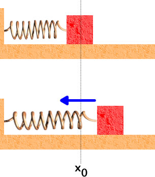It turns out that to a fairly good approximation, the force exerted by the spring is proportional to the distance from the equilibrium position. This is called Hooke's Law and mathematically is:

(7)

Here k is a constant for a particular spring. The first minus sign indicates that the force is restoring: if x is greater than x₀ the force is negative; if x is less than x₀ the force is positive. Thus the force always points towards the equilibrium position.

Newton taught us the relation between forces F, masses m and the acceleration a:

(8)

Combining these two equations gives the relationship between the acceleration and the position of the mass:

(9)

The constant c equals the spring constant divided by the value of the mass.

The acceleration is the rate of change of the speed. Thus, if the mass has an initial speed v_i then after a small time dt its final speed v_f is:

(10)

Similarly, the speed is the rate of change of the position, so:

(11)

We create a sphere instance of a sphere movie clip, just as in the Doing It With ActionScript section, and create an actions layer.

Here is the code in the actions layer implementing Equations 9, 10, and 11. The result is shown below.

Note that the ActionScript has no trig functions, and just increments the speed based on the current value of the acceleration and the position based on the value of the speed. However, it sure looks like the position is varying with time like a sine function.

There are some subtleties in the three simple lines of code that update the acceleration, speed and position. For example, as written we update the position x using the new value of the speed v. If we reverse the lines updating x and v we update the position with the old value of the speed:

	...
	a = -c * (x - x0);
	x += v * dt;
	v += a * dt
	...

One could also imagine updating the position using an average of the old and new values for the speeds. These subtleties are beyond the scope of this document: googling "Euler's method" can get you started on learning about them. There is also a small note about this and the above animation at the end of this section.

Also, Equations 10 and 11 are only true when the "time step" dt is infinitesimally small. Above I have set the time step to one over the frames per second of the animation, 1/12 = 0.08333... This is pretty small, but certainly not infinitesimally small.

We can increase the accuracy of the animation by putting a loop inside the onEnterFrame function to reduce the size of the time step used in doing the calculation. Here is some code which reduces the effective time step to 1/1200 = 0.00008333... :

onEnterFrame = function(){
	for(i = 1; i <= 1000; i++) {
		a = -c * (x - x0);
		v += a * dt/1000;
		x += v * dt/1000;
	}
	sphere._x = x;
}

Of course, this increases the number of computations that must be done for each frame by a factor of 1000. Assuming a reasonably fast computer, this modification has no visible effect on the animation, so I do not bother to display it.

Finally, although this technique of "numerical integration" doesn't have many benefits for the undamped oscillator there are circumstances, such as many problems in chaos, in which no analytic solution exists. In these cases numerical integration is often the only way to do the animation.

For example, the famous "three body gravitational problem" in which there are two fixed suns and one planet has no analytic solution. Clicking on the button to the right will show a numerical integration which solves this problem; file size is 50k and it will appear in a separate window.

Technical Note

Although this tutorial is about Flash and ActionScript, full disclosure requires that I mention a couple of points about the numerical integration of the undamped oscillator above. The Euler method referred to above updates the position using the old value of the speed, which is not the way the shown animation does it: in the animation we use the new value of the speed to update the position. For this problem, the actual Euler method is unstable for the step size that was used, and the amplitude of the oscillation increases forever. If we reduce the step size by a factor of 1000 using code such as is shown above, the Euler method is stable and the animation looks essentially identical to the one shown.

Numerical Approximation Homework

Here are a some problems for you to do.

Problem 1

For the undamped oscillator, modify the code so that the position is updated using the old value of the speed and observe the results. Inplement code similar to that shown above to decrease the step size by various amounts and see what happens.

Problem 2

As mentioned at the beginning of the Damped Harmonic Motion section, the damped harmonic oscillator that we animated above has a damping force that is proportional to the speed of the object:

Here is a constant for a given physical system, and the minus sign indicates that the damping force points in the opposite direction to the speed, so it always tries to slow the object down.

The total force acting on the object is the sum of this damping force and the force exerted by the spring given by Eqn. 7. This total force is equal to the mass times the acceleration, Eqn. 8.

Use numerical integration to produce an animation of damped harmonic motion.

Problem 3

The above damping force turns out to not be very realistic for most physical circumstances. A better approximation to the damping force is:

(12)

The force varies as the square of the speed, and b is a constant. The problem with this is that the solution is not analytic, which is why most introductory Physics courses use the simpler form.

Make an animation for this case using numerical integration.

About Versions of ActionScript

Recent versions of Flash MX and the Flash player support Version 2 of the ActionScript language. This allows one to program using object oriented methods. Although I am a big fan of this for big programming projects, nothing in this session uses object oriented methods.

Reference

This tutorial has only scratched the surface of this topic. There are many resources available to learn more about ActionScript, and I will not attempt to list them here.

However, if at the end of your Physics course you immediately threw your textbook into the lake, you may wish to refresh your memory about the Physics. Fortunately, there is a book designed just for you. Although the code fragments are C++, translating them to ActionScript is fairly trivial. The book is:

David M. Bourg, Physics for Game Developers (O'Reilly, 2002, ISBN 0-596-00006-5)

Author

This document was written by David M. Harrison, Dept. of Physics, Univ. of Toronto, harrison@physics.utoronto.ca, in January 2005. It was last modified on $Date: 2005/11/18 14:43:45 $ (y/m/d UTC).

This work is licensed under a Creative Commons License.