 Introduction to
Standing Waves
Introduction toThe phenomena of standing waves and resonance has been studied since at least the time of Pythagoras. In this document we introduce the Standing Waves and Acoustic Resonance experiment from the Physics laboratory at the University of Toronto. It is intended to be used before you begin the experiment. The Preparatory Questions at the end of this document should be answered and turned in to your Demonstrator before you begin to work on the experiment.
![]()
In order to effectively use this page, your browser needs to be capable of viewing Flash animations, also known as swf files. The Flash player is available free from http://www.macromedia.com/. Our animations are for Version 5 of the player or later.
You will also want to have either the Real Media or QuickTime video player installed on your computer. The Real Media player is available free from http://www.realnetworks.com/. The QuickTime player is available free from http://www.apple.com/quicktime/.
We have also prepared a copy of the soundtrack of the video and a summary of the information in this page. For most people, effectively using these will mean having it in hard-copy instead of reading it on-screen. Thus, they are prepared in pdf format. Accessing them will require that you have the Acrobat Reader, which is available free from http://www.adobe.com
![]()
In order to do the Standing Waves experiment, somewhat more background information is required than is typical for experiments in this laboratory. This section provides some of that needed background; the Possible Standing Waves section below provides more of the required background. It you are doing this experiment in the second term, the Energy Dissipation section will also supply you with some needed information.
| A brief non-mathematical introduction to standing waves, prepared for another context, exists. You may access an html version by clicking on the link to the right that says html; it has a file size of 189k. You may access a pdf version by clicking on the link that says pdf; it has a file size of 195k. Either version will appear in a separate window. You should choose the html version of this document if you are intending to read it in a browser; you should choose the pdf version if you intend to print it and read it in hardcopy. |
|
A sound wave is a longitudinal wave because the thing that is "waving," the molecules of air, are moving in the same direction as the wave itself. This is different from a transverse wave such as a wave on a string, where the thing that is waving, the string, is moving in a direction that is perpendicular to the direction of the wave's motion.
|
The above figure is a slow motion animation of a tuning fork generating a sound wave. The light gray regions represent a low density of air molecules; the dark gray represents high density. The low density regions have a pressure less than atmospheric pressure, while the high density regions have a higher pressure. If you are a Physics student at the University of Toronto you may have studied this relation between density and pressure in the Boyle's Law experiment. |
A graph of the pressure of the air at some moment in time as a function of position will be a sine wave. This sine wave is traveling from left to right in the figure. The pressure at zero amplitude of the wave is just atmospheric pressure. Later it will be important for you to know that microphones measure this pressure wave.
The speed of the sound wave varies with the temperature. The accepted value is:
| vaccepted = 331.4 + 0.61 t (m/s2) | (1) |
where t is the temperature in Celsius.
Just as for all waves, the sound wave travels through the air. The medium of the wave, the air molecules, vibrate back and forth but do not move off to the right with the wave. The molecules' vibration is sinusoidal. Therefore we also can characterise a sound wave in terms of the displacement from equilibrium of the individual air molecules.
|
It will be useful to think of a model where the air molecules are connected to each other by springs, as indicated in the above figure. |
|
A Flash animation of the oscillations of the air molecules has been prepared. It may be accessed by clicking on the green button to the right. The animation will appear in a separate window, and the size of the animation file is 20k. |
Some key points in the animation are that:
| Pauses the animation | |
| Resumes the animation | |
| Step forward one "frame" | |
| Step back one "frame" |
In conclusion, where the amplitude of the pressure wave is a maximum or minimum the amplitude of the displacement wave is zero, and vice versa. This is indicated in the following figure.
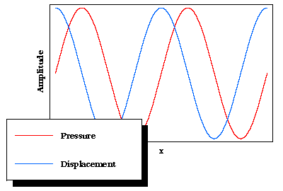
In most of what follows, we will be analysing the displacement wave. You need to remember that the microphone you will use to measure the wave measures the pressure wave.
Consider a sound wave incident on a barrier that reflects it. The air molecule that is just next to the barrier can not move to the right, so the amplitude of the displacement wave must be exactly zero at that position. The air molecule just to its left collides with the barrier elastically, and rebounds by moving to the left. So in terms of the displacement sound wave, the reflected wave has the opposite orientation to the incident wave: if the incident wave has a positive amplitude the reflected wave has a negative amplitude, and vice versa.
|
A Flash animation of an incident displacement sound wave reflecting off a barrier may be accessed by clicking on the red button to the right. The animation will appear in a separate window, and has a file size of 41k. You will see that it has "playback" controls to stop and start the animation. |
The positions in the animation indicated by the blue lines are called nodes; at these points the sum of the two waves is always exactly zero. The points half-way between the nodes where the amplitude becomes a maximum or minimum value are called antinodes. Of course, a node in the displacement wave shown in the animation is an antinode in the pressure wave.
The distance between the nodes of the sum of the two waves is exactly one-half of the wavelength of the incident and reflected wave. You can see this more clearly in the animation by clicking on the Pause button.
If we have a wave traveling from right to left and reflecting off a barrier, the picture would be just the mirror image of the animation.
Now, imagine we have two barriers, and a sound wave is reflecting back and forth between them. If the left-hand barrier is placed at the position of one of the nodes of the situation shown in the animation we looked at above, then the wave reflected off the left-hand barrier will exactly match the wave traveling from left to right.
|
An animation of this may be accessed by clicking on the blue button to the right. It will appear in a separate window, and has a file size of 41k. |
Thus if the left-hand barrier is at one of the nodes in the total wave produced by the right-hand barrier we form a standing wave. Note that if the left-hand-barrier were not placed at a node, then its reflected wave would not lie on top of the wave incident on the right-hand barrier, so a standing wave would not be formed.
As you can see, if d is the distance between the nodes, it is
related to the wavelength
![]() of the waves that form the standing wave
as:
of the waves that form the standing wave
as:
| (2) |
Formation of standing waves is sometimes called resonance.
Here is a summary of the material in this sub-section:
![]()
|
In order to perform the experiment you will need to know how to use an oscilloscope. An introduction to this instrument may be accessed by clicking on the yellow button to the right. It will appear in a separate window, and has a file size of 42k. |
We have prepared a video in various formats to introduce you to the apparatus; the running time of the video is about 6:30 minutes. Links to the video appear below. You will wish to adjust the volume of the speakers on your computer so that you can easily hear the soundtrack.For the higher resolution RealMedia version, you may also wish to increase the size of the video using the controls provided by the player.
| You may download a pdf version of the soundtrack of the video by clicking on the green button to the right. It will appear in a separate window, and has a file size of 76k. |
The Streaming video will be played by the RealMedia player as it is delivered to your computer by the network. The Download versions of the video will be downloaded to a temporary area on your local hard disc and then shown if your browser is configured to use the appropriate player. You may save these Download versions to a more permanent place that you specify on your computer's discs by right clicking on the link and then saving the Target (Internet Explorer) or Link (Netscape)
|
|||||||
|
|||||||
| There is a diagram of the apparatus, which may be accessed by clicking on the blue button to the right. It will appear in a separate window, and has a file size of 37k. You may wish to print this diagram. If so you will probably need to use landscape mode for the printout. |
You should treat the representation of the Signal Generator and Oscilloscope in the diagram as generic; the instruments you use may look different from those shown.
![]()
In the Introduction we considered the placement of two barriers so that a given sound wave would set up a standing wave between them. In the actual experiment, the left-hand "barrier" is the loudspeaker that generates the sound wave; the fact that the face of the loudspeaker is vibrating back and forth may be ignored.
We now consider the placement of the barriers to be fixed, as in the experiment, and ask what frequencies and wavelengths of a sound wave reflecting back and forth between them will form a standing wave. The answer is any wavelength where the nodes of the displacement standing wave correspond to the position of the barriers.
|
An animation of the three largest wavelengths that produce standing waves for a fixed position of the barriers may be accessed by clicking on the orange button to the right. It will appear in a separate window, and the file size is 9.2k. |
|
Note that the wavelengths all match the equation: |
(3) |
where L is the distance between the two barriers.
Although the animation only shows values of n equal to 1, 2, and 3, the equation correctly indicates that there are an infinite number of possible standing waves corresponding to the infinite number of positive integers.
The animation correctly shows that the frequency of different standing waves are different.
|
The wavelengths are related to the frequency f of a wave traveling at a speed v according to: |
(4) |
Equation 4 is true for all waves.
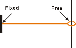
It may surprise you to learn that if the right-hand barrier is removed so that the tube is open to the air, standing waves are still set up for appropriate values of the frequency and wavelength of the sound wave. The major difference is that at the right-hand side there in an antinode is the displacement wave instead of a node.
|
An animation of the first three possible standing waves with one end of the tube open may be accessed by clicking on the green button to the right. The animation will appear in a separate window, and the file size is 16k. |
You may have noticed that the length specified in the animation is not just the length L of the tube, but is an effective length Leff. The effective length is given by:
| Leff = L + 0.3 D | (5) |
where D is the diameter of the tube.
Sometimes Leff is called the acoustic length.
These standing waves are also the ones for a string that is fixed at one end and free to move up and down on the other end. The "free" end can be realised by ending the string with a loop around a vertical frictionless rod, as shown to the right. |
 |
Although the animations illustrate the formation of standing waves, to derive that such waves are actually formed involves writing down the mathematical formulation for a traveling wave moving from left to right and the equation for another traveling wave moving from right to left, with the phase relationship between the two waves such that it correctly describes the behavior where the reflection occurs. Then the sum of the two equations may be manipulated into the equation of a standing wave. Such manipulations are not part of this experiment. Instead they are part of theoretical physics, which is the subject of the lecture component of your physics course. The laboratory is teaching the "better half" of physics: experimental physics.
One of the factors that will influence the quality of your data is how well you have adjusted the frequency of the sound wave to achieve a good resonant standing wave. Here is a brief prescription:
![]()
Whe done as a first term Core experiment, this section describes the experiments to be performed.
Connect the output of the signal generator to the oscilloscope. Generate a voltage of a few hundred Hz and display it on the oscilloscope. In order for the display to be stable, you will want to trigger the oscilloscope on the input voltage.
If you have not used an oscilloscope before this may take a few minutes; this part, then, is your opportunity to begin to learn how to use this instrument.
|
Remember the recommendation in the web-document on using an oscilloscope: first take a few moments to locate the major controls on the instrument. Randomly turning knobs and flipping switches is almost certain to not produce the display that you desire. |
The relationship between the frequency f, in Hz, and the period T, in seconds, is:
f = 1/T |
(6) |
Compare the frequency of the wave as read by the signal generator to the frequency as measured by the oscilloscope.
Connect the output of the signal generator to the loudspeaker. Connect the output of the microphone to the second beam of the oscilloscope and adjust the display so that you can see both the input voltage from the signal generator and the output of the microphone simultaneously.
You should be able to hear the sound wave if you place your ear near the tube.
Have the tube closed at both ends. For some frequency between, say, 200 Hz and 2 kHz, adjust the frequency so that a standing wave exists in the tube.
Question: how does the sound level that you hear with your ear close to the tube correlate with whether or not a standing wave exists in the tube? Can you think of why this is so?
For the lowest frequencies, the maximum amplitude as measured by the microphone does not occur at the position of the loudspeaker, but a noticeable and measurable amount down the tube away from it. This is your first indication that the simple picture of these waves as described above is not quite complete
From the positions of the nodes and/or antinodes, determine the wavelength of the standing wave. Calculate the speed of sound. Repeat for a few different frequencies. Give a final best value for the speed of sound and compare your result to the accepted value.
For one of the higher frequency standing waves, from your measurements of the wavelength determine the length of the tube. Compare to a direct measurement of the length. Are they the same within errors?
Open one end of the tube, and adjust the frequency for a standing wave. The standing waves in this case will correspond to the standing waves on a string with one end free to move. From the speed of sound, the frequency of the wave, and your measurements of the positions of the nodes and/or antinodes, calculate the length of the tube and compare to your result of Part 1.
Above we discussed the effective length of the tube when one end is open, whose value is given by Equation 5.
Does your data confirm Equation 5? A simple answer of "yes" or "no" is not sufficient: you must prove your answer using your data.
![]()
So far we we have discussed the Standing Waves experiment as it is done in the first term. In the second term you will, of course, be a more proficient experimentalist capable of more thorough investigations. This section provides background information that will be needed for doing the experiment in the second term.
If you think for a moment about the situation discussed above where the loudspeaker is generating a sound wave and the right-hand side of the tube is open, it should be clear that the loudspeaker is continuously putting out sound energy, most of which escapes into the room.
Even if the right-hand side of the tube is closed the system still dissipates energy into the room, since you can hear the sound.
The Quality Factor Q is related to the dissipation of energy. A higher value means that the system loses a smaller fraction of its energy to the surroundings.
|
Imagine we have a standing wave when the frequency f0 is 50 Hz. We place the microphone at a position where it measures a maximum, an antinode in the pressure wave. Then if we slowly change the frequency to values either less than or greater than 50 Hz, the amplitude measured by the microphone will decrease as we get further away from resonance. A plot of amplitude versus frequency is shown to the right. In the figure we assume that the amplitude at resonance is one. |
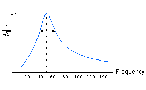 |
In the figure we indicate the full width of the curve when the amplitude
is 1/![]() 2 ( ~ 0.707) times the maximum amplitude
2 ( ~ 0.707) times the maximum amplitude
|
We shall call that width |
Then the Quality Factor Q is approximately:
| Q = f0 / |
(7) |
![]()
In addition to Parts 1 and 2 above, in the second term you should also do this part of the experiment.
Close the tube at both ends and adjust for a standing wave in the range of 200 Hz - 1 kHz. Place the microphone at a maximum in the pressure wave and take data for the amplitude as a function of frequency for frequencies close to the resonant frequency.
Calculate the Quality Factor of the tube.
![]()
These questions should be answered and turned in to your Demonstrator before beginning the experiment. They are almost the same questions that appear in the Guide Sheet, except that the equations in this document are numbered differently than in the Guide Sheet; here the numbers refer to this document.
![]()
As promised at the beginning, we have prepared a summary of the information presented above. It does not attempt to provide a full discussion, but just reviews the "high points" from above.
| You may access the summary by clicking on the red button to the right. The summary is in pdf format, will appear in a separate window, and has a file size of 29k. You may wish to print this document. |
![]()
Earlier versions of this Guide Sheet have been worked on by Joe Vise (1989) and David Harrison (1999 and 2001).
This web version is by David M. Harrison, May, 2003.
This is $Revision: 0.1 $, $Date: 2003/05/09 14:53:11 $ (y/m/d UTC).