Least Squares Fitting of Data from the Physical Sciences & Engineering
Solomon R.C. Douglas and David M. Harrison, Dept. of Physics, Univ of Toronto.
This document is based on a contributed paper given at the Maple Summer Workshop, Wilfrid Laurier University, Waterloo Ontario, in July 2004.
Introduction
We have been developing a least-squares linear fitter written in Maple. We will discuss the design principles that we believe are important for a fitter to be used for analysis of data from the physical sciences. We will illustrate with both real-world and synthetic datasets.
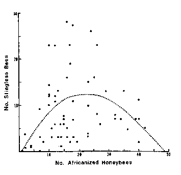
The figure to the right is from a study of the genetics of bees which was published as
David W. Roubik, Science 201 (1978), 1030.
Despite the fact that the paper passed the rigorous review process of the prestigious journal Science, it seems immediately obvious that the fitted polynomial looks nothing like the data. In fact I think the data looks more like a duck, with the beak pointing to the left in the upper-left quadrant.
The point to this illustration is not to heap abuse on either the author or reviewers, but to point out that given inappropriate tools and inadequate background many smart people will make such errors.
| Clicking on the blue button to the right will access a little Flash animation I put together on a quiet afternoon. It will appear in a separate window and has a file size of 13k. |
|
|
 |
| Figure Caption: "The dashed line is a quadratic polynomial (given by y = -0.516 + 1.08x - 0.23x2) which gave the best fit to the points." |
|
Numerics Are Not Enough
F.J. Anscombe devised 4 datasets which were published in American Statistician 27 (Feb. 1973), 17. Each dataset consists of 11 ( x, y) pairs.
The means of the values of x and y are almost identical for all 4 datasets:
| |
Mean of x |
Mean of y |
| Set 1 |
9.00000 |
7.500909091 |
| Set 2 |
9.00000 |
7.500909091 |
| Set 3 |
9.00000 |
7.500000000 |
| Set 4 |
9.00000 |
7.500909091 |
If we fit each dataset to a straight line using least-squares techniques, ignoring the question of significant figures the results are:
| |
Intercept |
Slope |
Sum of the Squares |
| Set 1 |
3.000090907 ± 1.124746791 |
.50009090919 ± .1179055006
|
13.7627 |
| Set 2 |
3.000909089 ± 1.125302416 |
.50000000010 ± .1179637460 |
13.7763 |
| Set 3 |
3.002454546 ± 1.124481230 |
.49972727260 ± .1178776623 |
13.7562 |
| Set 4 |
3.001727277 ± 1.123921072 |
.49990909030 ± .1178189417 |
13.7425 |
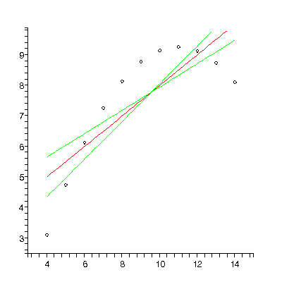
| The point is that the numerical analysis could easily lead us to the conclusion that the 4 datasets are very similar. However, if we examine plots of the data it becomes clear that this is not true. Clicking on the blue button to the right will illustrate in a separate window. |
|
Here is the output of the fitter we are developing for Set 2:
|
TABLE([0 = [3., 1.1], 1 = [.50, .12]]), 13.8, 9 |
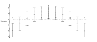
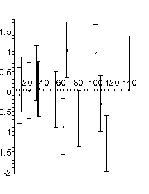
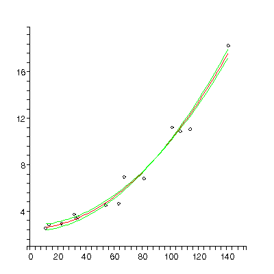
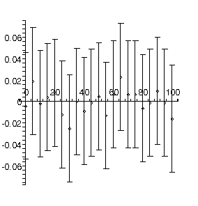
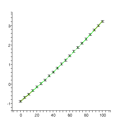
The upper-left plot shows the residuals, which clearly shows that the data do not correspond to a straight-line relationship. This is also shown in the upper-right plot, which shows the data and the results of the fit. In this plot, the red line is the fit result and the green lines show the effect of the estimated errors in the fitted parameters. Below are the numeric results of the fit. The entry 0 = [3., 1.1] is the value and error of the zeroth power, i.e the intercept. The 1 = [.50, .12]] is the value and error of the slope. This is followed by the sum of the squares of the residuals for the fit, 13.8, and the number of degrees of freedom, 9.
For a good fit using an appropriate model, we expect the residuals to be randomly distributed about zero: whenever the residuals show a trend, as in the above plot, it is likely that the model is not appropriate for the data.
You may notice that the significant figures of the values and errors of the fitted parameters are different from the values in the previous table. We will discuss this later.
You may also notice that error bars are shown in the residual plot. Our fitter by default applies a statistical assumption to estimate errors in the data, and these are what are shown; this assumption may be turned off with an option.
Estimated Errors in the Fitted Parameters Are Necessary
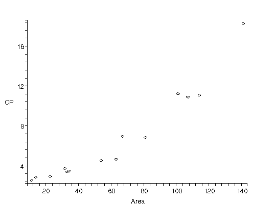
The figure to the right is from Barry Lia, Robert W. Williams and Leo M. Chalupa, Science 236 (1987), 848. It is data for the ratio of the central ganglion cell density to the peripheral density (CP) versus retinal area for 14 cat fetuses.
The authors fit the data to a straight line and from the slope and intercept attempted to deduce information on how the retina develops!
|
 |
| In the previous section we pointed out that even if the authors ignore the fact that the plot of the data indicates that a straight-line fit is not appropriate, a plot of the residuals of the fit would make this fact harder to ignore. The figure to the right is the residual plot of the straight-line fit by our fitter, and the "happy face" is hard to miss. |
 |
In analysing this data, adding a quadratic term seems reasonable. Here is the numeric result of that fit:
TABLE([0 = [2.91, .58], 1 = [-0.13e-1, 0.20e-1], 2 = [0.84e-3, 0.13e-3]]), 5.52, 11
This indicates that the slope of the fit is -0.013 ± 0.020. But this is zero within the estimated uncertainty in the value. Thus a more appropriate fit is to a parabola without a linear term.
In a moment we will also want to use the fact that the sum of the squares of the residuals divided by the number of degrees of freedom of the fit is 5.52/11 = 0.502.
Here is the result of fitting this dataset to a parabola:
|
TABLE([0 = [2.56, 0.25], 2 = [0.000757, 0.000032]]), 5.75, 12 |
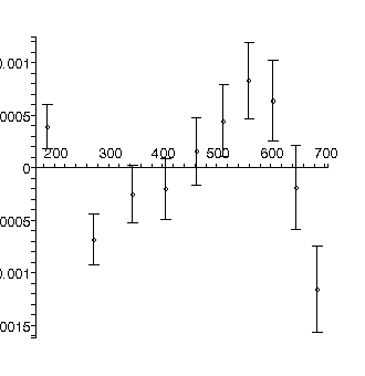
Now the residuals appear to be randomly distributed about zero, as they should for fitting the data to an appropriate model. Note that not all residuals are zero within the estimated errors: this is consistent with a good fit. In fact, if the errors are standard deviations we only expect about 67% of the residuals to be zero with errors.
The values of the fitted parameters for the intercept and the quadratic term have been significantly shifted by dropping the linear term, and errors in those parameters have been reduced.
Also, the sum of the squares of the residuals divided by the degrees of freedom is now 5.75/12 = 0.479, which is less than the value of 0.502 when we included the linear term: this also increases our confidence that this fit is appropriate for the data. We will discuss the significance of this in more detail later.
The main conclusion of this section is that it was the errors in the fitted parameters that were returned by the fitter that led us to, apparently correctly, drop the linear term in the fit.
There is a small technical matter about the last fit to the ganglion data, which we will point out but not discuss in this document. The residual plot seems to indicate that as the value of the independent variable increases, the magnitude of the residual also increases. This indicates that a transformation of the data could yield better information.
Information of the Quality of the Fit
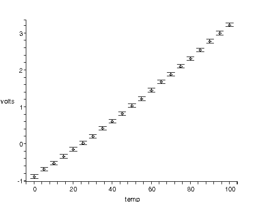
The figure to the right shows voltage versus temperature data for the calibration of a thermocouple. The data were taken by a student, and presented in the classic Philip R. Bevington, Data Reduction and Error Analysis (McGraw-Hill, 1969), 138.
The plot was produced by a function developed in conjunction with our fitter, and shows the experimenter's specification of the error in the voltage.
Note that for unexplained reasons the student did not provide errors in the temperature. |
 |
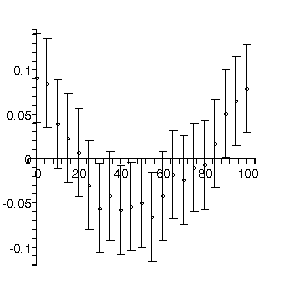
We fit the data to a straight line. The residual plot and numerical results are shown to the right.
Again, the residuals indicate that we need to at least add a quadratic term to the fit. The error bars shown in the residual plot are the values from the data.
Because there are explicit errors in the dependent variable, the voltage, the numeric information returned by the fitter includes that chi-squared, 21.1, instead of the sum of the squares of the residuals. This number is essentially the sum of the squares weighted by the stated errors. |
|
TABLE([0 = [-.981, 0.021], 1 = [0.04122, 0.00036]]), 21.1, 19
|
|
In the previous section, we were looking that the sum of the squares of the residuals divided by the degrees of freedom of the fit. We pointed out that a smaller value of this ratio indicated that the model being used matched the data more closely.
For this fit to data with explicit errors, the analog is the ratio of the chi-squared to the degrees of freedom is 21.1/19 = 1.11. If this ratio were big, then we can conclude that the fit is poor. However, if the ratio is too small then the fit is too good to be true. It turns out that the ideal value of the ratio is about 1.
Fitting the data to a quadratic gave the following result:
|
TABLE([0 = [-.886, 0.30e-1], 1 = [0.352e-1, 0.14e-2], 2 = [0.60e-4, 0.13e-4]]), 1.01, 18 |
There are 2 related problems with this fit:
- The chi-squared, 1.01, divided by the degrees of freedom, 18, is much less than 1.
- All of the residuals are easily equal to zero within errors. As discussed earlier, in the ideal case only about two-thirds of the residuals should be zero within errors.
Examining Bevington's discussion of the data we learn that the given errors in the voltage were just guesses by the student. We now conclude that those guesses were much too pessimistic about the accuracy and precision of the data.
Real Data Have Errors in Both Coordinates
In the previous section we chided the student who did the thermocouple calibration for not estimating errors in the temperature as well as the voltage. In his defence, although some but not all fitters allow for explicit errors in the dependent variable very few fitters allow for errors in both coordinates. Perhaps the student knew that nothing could be done with an error in the temperature.
Of course, our fitter handles this case.
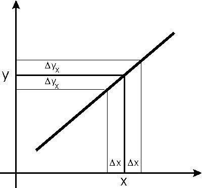
Because this effective error depends on the derivative of the function to which we are fitting the data, using this technique requires that the fitter iterate to a solution, so convergence criteria must be used to decide when the iterations should be stopped.
In addition, there is some subtlety in deciding what value of the independent x coordinate should be used in evaluating the derivatives. For more details see Matthew Lybanon, American Journal of Physics 51 (1984), 22.
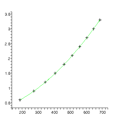
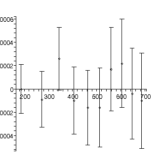
We will use our fitter to fit data taken from a free fall experiment in a teaching laboratory in the Dept. of Physics at the Univ. of Toronto. The data include explicit errors in both the distance and time coordinates. In the absence of air resistance we expect the distance to fit to a quadratic in the time. Here is the result of such a fit:
|
TABLE([0 = [.19139, 0.66e-3], 1 = [0.13116e-2, 0.35e-5], 2 = [0.47128e-5, 0.42e-8]]), 31.3, 7 |
The residuals show that the model is not appropriate: this is because for this apparatus the effects of air resistance are not negligible. This is also reflected in the fact that the chi-squared of 31.3 is much larger than the degrees of freedom, 7.
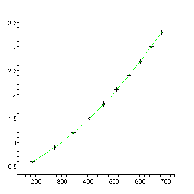
We fit again adding a cubic term:
|
TABLE([0 = [.2009, 0.19e-2], 1 = [0.1228e-2, 0.16e-4], 2 = [0.4930e-5, 0.41e-7], 3 = [-0.172e-9, 0.32e-10]]), 2.34, 6 |
Roughly, the value of the quadratic parameter, 0.000004930 ± 0.000000041, should be 1/2 of the acceleration due to gravity g in units of meters per millisecond-squared. Actually it is not quite this simple because g also appears in the value for the cubic term, but this is usually negligible.
Too Many Digits Are Hard To Read
Earlier we stated that fitting the first of Anscombe's datasets to a straight line gave an intercept and slope of:
- Intercept: 3.000090907 ± 1.124746791
- Slope: .50009090919 ± .1179055006
If we use our fitter to fit this dataset of a straight line it returns the values:
- Intercept: 3.0 ± 1.1
- Slope: 0.50 ± 0.12
We will discuss why in the usual case the fitter has done the right thing.
Consider for a moment the statement that some value is 1.2345 ± 0.6789. This statement says that we believe that value is between 1.2345 - 0.6789 and 1.2345 + 0.6789, i.e. between 0.5556 and 1.9134. However, if the claimed error is one of precision, say a standard deviation, then we are actually saying that the true value is probably in the claimed range. A moment's reflection will convince you that the specified range, (0.5556, 1.9134), has digits which have no possible physical significance. In fact, a more realistic specification of the range is something like (0.56, 1.91) or even (0.6, 1.9). This means that the original specification of 1.2345 ± 0.6789 can properly be written 1.23 ± 0.68 or perhaps 1.2 ± 0.7.
Our fitter by default does such significant figure adjustment based on the assumption that only 2 digits of the error are significant. This behavior can be controlled with an option.
Values of fitted parameters are usually much easier to read and interpret without all those non-significant digits being displayed.
Conclusions
For least-squares fitting of data from the physical sciences and engineering, we have argued that:
- Fitting data is sometimes surprisingly subtle.
- Displaying graphical information (residuals, data and fit results) is important.
- Calculated errors in the fitted parameters should be returned.
- Information on the quality of the fit (sum of the squares of the residuals or chi-squared, number of degrees of freedom) should be returned.
- Errors in both coordinates of the data should be handled correctly.
- The errors in the fitted parameters should be used to do significant figure adjustment on the values.
Copyright
This document is Copyright 2004 David M. Harrison
|
