The Free Fall Experiment

In this document we introduce the Free Fall experiment from the Physics laboratory at the University of Toronto. It is intended to be used before you begin the experiment. The Preparatory Questions at the end of this document should be answered and turned in to your Demonstrator before you begin to work on the experiment.

Requirements

In order to effectively use this page, your browser needs to be capable of viewing Flash animations, also known as swf files. The Flash player is available free from http://www.macromedia.com/. You will need Version 6 or later of the player.

We have also prepared a summary of the information in this page in a pdf format suitable for printing. Accessing this document will require that you have the Acrobat Reader, which is available free from http://www.adobe.com

Introduction

The "modern" study of objects in free fall near the Earth's surface was begun by Galileo some 400 years ago.

In this experiment you will use the free fall of an object to determine the acceleration due to gravity g.

A secondary goal of the experiment is to study the effect of air resistance.

When an object is in free fall near the Earth's surface, then if air resistance is negligible we can relate the distance s the object falls in a time t to its initial position s₀ at time t = 0, the initial speed v₀ at time t = 0, and the acceleration due to gravity g according to:

(1)

If you fit distance s versus time t to a second order polynomial ("powers" of 0, 1, 2 in the language of the fitter), the fit is to:

(2)

The fitter will return values and errors for a₀, a₁ and a₂. a₀ is the value of the initial position, a₁ the value of the initial speed, and a₂ one-half of the value of g.

The apparatus for this experiment is sufficiently precise that for some objects air resistance is not negligible. The air resistance exerts an upward force, which causes an upward acceleration on the object.

(3)

The upward acceleration due to the air resistance depends on the speed squared and a constant . depends on the size and mass of the object and on its surface roughness and shape. The acceleration is approximately equal to:

(4)

In this case the simple relation between distance and time becomes more complex. A reasonable approximation of the solution to the equations of motion is:

(5)

The important thing to notice here is that the distance s now depends on four terms involving the time t: a term that is independent of the time, a term that is linear in time, a term that depends on the time squared, and a term that depends on the time to the third power. Thus if air resistance it not negligible, you will fit you data the a third-order polynomial:

(6)

The fitter will return values and errors for the coefficients a₀ , a₁, a₂ and a₃. You may then determine the values and errors of s₀, v₀, g and in Equation 5.

Deriving Equation 5 involves first setting up the equation of motion using Newton's Second Law including the air resistance term Equation 4. Then one solves the differential equation with suitable initial conditions. This sort of mathematical manipulation is an example of theoretical physics, which is what you study in the lecture component of your Physics course. In the laboratory we are not teaching theoretical physics, but experimental physics. Thus we simply accept Equation 5 as having been correctly derived by a theorist. In this case, the derivation is beyond the level of the typical first year physics course.

Apparatus and Data Collection

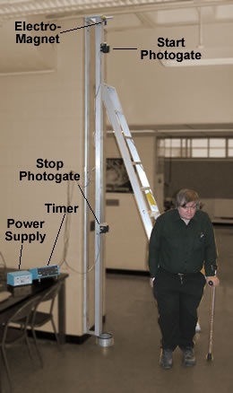
The photograph to the right shows the apparatus for the Free Fall experiment. An aluminum track has an electromagnet mounted at the top. It also has two photogates mounted on it whose vertical position can be changed. The track is over 3 meters long. Lab technologist Rob Smidrovskis is standing beside the apparatus to help give you a sense of the size. You will suspend an object from the electromagnet. A Release button on the Power Supply cuts the power to the magnet and drops the object. When the object falls through the upper Start Photogate it start the Timer. When it falls through the lower Stop Photogate it stops the timer. A container on the floor catches the fallen object.

Here is a simulation of the Free Fall apparatus. The drawing is not to scale, and we have also slowed down time.

The object is suspended by an electromagnet. Clicking on the Release button turns off the current through the magnet and the object starts falling. When it passes through the upper Start Photogate and breaks the light beam, the timer starts. When it passes through the lower Stop Photogate, the timer stops. Clicking on the Reset button resets the timer. In the simulation it also places the object back onto the magnet: in the actual experiment you will do that yourself. In the actual experiment, the apparatus is so sensitive that repeating a measurement without moving the photogates will usually give values of the time that are slightly different. The behavior is duplicated in the simulation. You will keep the position of the upper Start Photogate fixed throughout the experiment, so the initial speed of the object v0 remains constant. You will move the position of the lower Stop Photogate to different positions to vary the distance s the object falls. The value of the distance s is the distance between the light beams of the two photogates. If the simulation does not work, it is likely you have an older version of the Flash player. This page requires Version 6 or better of the player.

Although the distance s is the distance between the light beams of the photogates, that is not what you will measure. Each photogate has a viewport which allows you to see the metal scale mounted on the track underneath. Since each photogate is constructed identically, reading the positions of each gate with the viewport is equivalent to determining the positions of the light beams of the two gates. You will need to know that the manufacturer of the metal scale quotes a precision of one part in 4000.

There is more than one type of object available for use with the Free Fall apparatus:

• A streamlined metal bob. For this object the effects of air resistance are least.
• A light plastic sphere. A small metal plug is inserted so that it may be suspended from the magnet.

We can also supply a variety of ball bearings and other objects if you wish to experiment.

The photogates are moved by unscrewing a large knob on the back, moving the gate to a new position, and screwing the knob back in. When screwing the knob in, make it only finger tight. It is easy to screw the knob in too tightly and damage the apparatus.

Above we mentioned that the upper Start Photogate should remain in the same position for all the data. It should be placed about 10 centimeters below the bottom of the streamlined bob when it is suspended by the magnet.

You should place the lower Stop Photogate at 10 or so different positions. Be sure to make the range of distances s include the maximum value allowed by the apparatus. The minimum value of s should be about 10 cm.

For every position of the lower gate it is a good idea to take data for both the streamlined bob and the plastic sphere at once. This will save you some time and effort.

When you are using the streamlined bob, it is almost impossible to hang it from the magnet without it oscillating. Be sure to wait until the oscillations completely stop before dropping the bob. Otherwise, at best your data will be corrupted. At worst, the bob can hit one of the photogates, possibly damaging it.

You may be wondering why we use two photogates to start and stop the timer, instead of starting the timer when we turn off the current to the magnet and stopping the timer with a single photogate. The major problem is that when we turn off the current to an electromagnet the magnetic field does not go instantaneously to zero: the Free Fall apparatus is sufficiently sensitive that the time delay between turning off the current and the object beginning to fall will mess up the data.

Data Analysis

Taking the data for this experiment is fairly straightforward. However, because of the high precision of the apparatus, careful analysis of your data will be necessary. Here we discuss some of the issues of data analysis for this experiment.

The Dataset

The data analysis system on our computer allows you to create a dataset with up to 8 different variables. Each variable has a name which you assign when you create the dataset. You will probably find it convenient to define a single dataset for your data including values for both the streamlined bob and the plastic sphere. The variables could be:

• The distance between the photogates s.
• The time for the streamlined bob to fall through the gates.
• The time for the plastic sphere to fall through the gates.

When the program prompts you for the names of the variables in the dataset you should choose a descriptive name. The name should begin with a lower-case letter, and should contain only letters of the alphabet.

For example, here is a screen shot where what you might type is in boldface:

Enter your variables names and press RETURN: dist tBob tSphere

If the errors in the quantities are not the same value for all the datapoints, you will want to enter them into the dataset at this time too. If you have non-constant errors in all three variables you might set up the dataset variable names like this:

Enter your variables names and press RETURN: dist errdist tBob errBob tSphere errSphere

You will then enter the data in the order in which you named the variables, one set of six numbers per line.

Evaluating a Fit

Here we briefly review the material in the DATA FITTING TECHNIQUES in the lab manual. You should look over that material for a more complete description.

All good fitters, including ours, will return a value called the chi-squared, ². It measures how closely the fitted values match the data. A smaller chi-squared means the fit is closer to the data. The value is weighted with one over the values of the errors in the datapoints. Thus if the errors are large, the chi-squared is small; if the errors are small, the chi-squared is large.

The degrees of freedom of a fit is the number of datapoints minus the number of parameters to which you are fitting. Our fitter reports this number too.

The ideal value of the chi-squared is roughly equal to the number of degrees of freedom. If your chi-squared is not on the order of the number of degrees of freedom, there are three possibilities:

1. The model you are using is not appropriate. For example, if air resistance is significant and you are fitting distance versus time to only a second-order polynomial then the fit does not include the effects of air resistance. This would make the chi-squared too high. In this case you could try adding a third-order term to the polynomial.
2. You have been too optimistic in assigning errors to your data.
3. You have been too pessimistic in assigning errors to your data.

Another tool for evaluating a fit involves the residuals of the fit. These are the numeric values of the difference between the fitted values and the actual data values. For a good fit, the residuals should be randomly distributed around zero. If the model you are using is not appropriate for the data, the residuals will often show systematic deviations from zero.

For example, here are the residual plots for real data from the Free Fall experiment. The fit on the left was to a second-order polynomial; the other was to a third-order polynomial.

For this experiment, there is still another approach to determine if the effects of air resistance can be ignored. If you fit the distance versus time to a third-order polynomial, if air resistance is negligible the coefficient of the term for time to the third power will be zero within errors. In this case you can repeat the fit without including the third-order term.

This is a general principle of least-squares fitters: fitted values that are zero within errors should almost always be excluded from the fit.

Preparatory Questions

We hope that the following questions will guide you in your preparation for the experiment you are about to perform. They are not meant to be particularly testing, nor do they contain any "tricks". Once you have answered them, you should be in a good position to begin the experiment.

1. Call the positions of the two photogates s₁ and s₂.What are the reading errors in these quantities? The distance s is the difference between these two values.
2. What, then, is the error in s in terms of these errors? Now add in the error in the metal scale, 1 part in 4000, in quadrature to give an expression for the total error in s.
3. The accuracy of the timer is within its reading error of 0.05 msec. How can you determine whether the error of precision of your measurements of the time of fall is greater than 0.05 msec? Hint: the answer can only be determined by using the apparatus.
4. How can you estimate the speed of the object when it enters the first photogate before actually taking any data?
5. When an object is falling through the air, the terminal speed is the maximum speed it will reach.The terminal speed of a person is about 50 meters / second, depending on the individual and especially their orientation. What is their value for as defined in Equation 3?
6. If air resistance is not negligible, Equation 5 relates the distance to the time and the coefficient of air resistance . Here is that equation again:
   
   Meanwhile, if you fit distance versus time to a third-order polynomial, the fit is to:
   
   and the fitter will give values and errors for the coefficients a₁, a₂ and a₃. Write the equations that will allow you to determine v₀ , g and in terms of a₁, a₂ and a₃.

   

Summary

A summary of this document in pdf format has been prepared. You can print this summary to bring in to the laboratory if you wish. You may access the summary by clicking on the red button to the right. The file size is about 80k.

This experiment was originally designed and fabricated by Dr. Eustace Mendis when he was here in the early 1970's. The apparatus and Guide Sheet have been revised since then by David M. Harrison, Tony Key, Ruxandra Serbanescu, Rob Smidrovskis, Joe Vise, Taek-Soon Yoon and others.

This web version is by David M. Harrison, April 2003.

This is $Revision: 0.5 $, $Date: 2003/05/27 19:25:37 $ (y/m/d UTC).